Plot optimized matrix or optimization gipsmult object

Plot heatmaps of the MAP covariance matrices estimator or the convergence of the optimization method. The plot depends on the type argument.

Usage

# S3 method for class 'gipsmult'
plot(
  x,
  type = NA,
  logarithmic_y = TRUE,
  logarithmic_x = FALSE,
  color = NULL,
  title_text = "Convergence plot",
  xlabel = NULL,
  ylabel = NULL,
  show_legend = TRUE,
  ylim = NULL,
  xlim = NULL,
  ...
)

Arguments

x

Object of a gipsmult class.

type

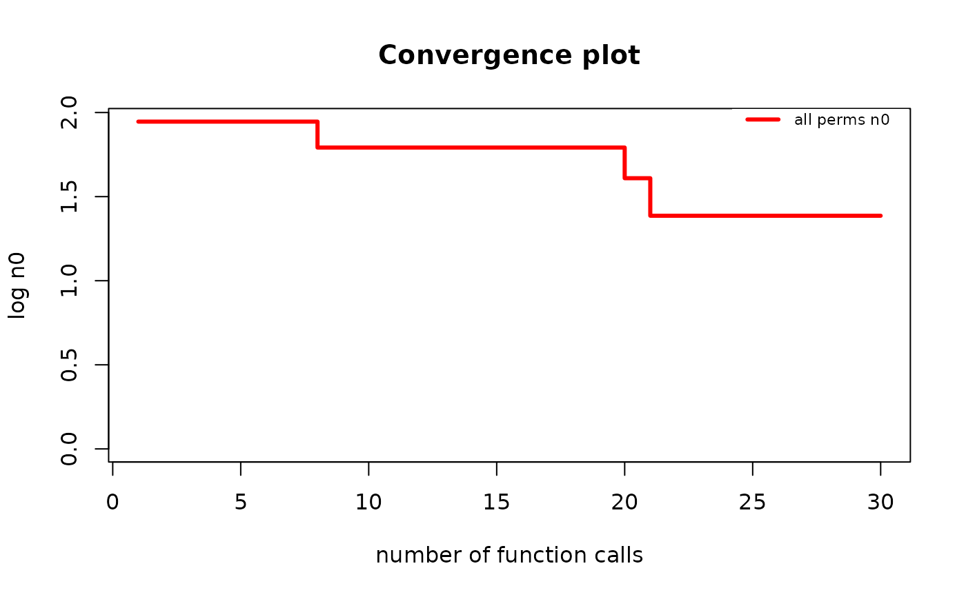
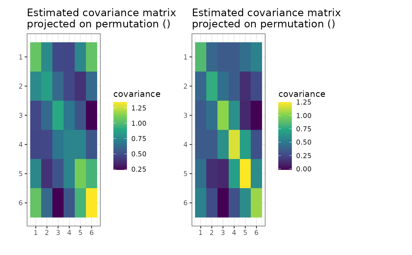
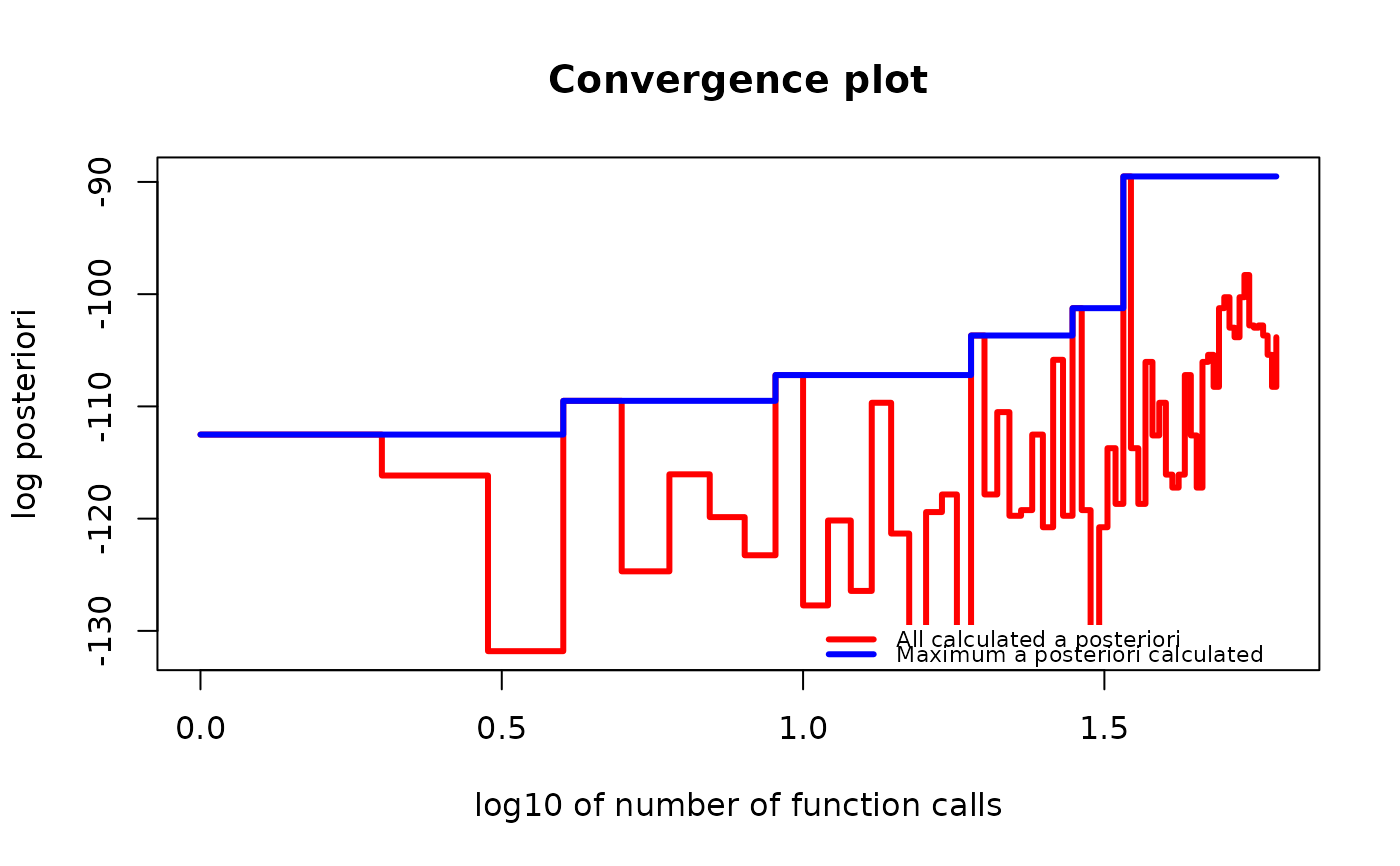
A character vector of length 1. One of c("heatmap", "MLE", "best", "all", "both", "n0", "block_heatmap"):

"heatmap", "MLE" - Plots heatmaps of the Maximum Likelihood Estimator of the covariance matrices given the permutation. That is, the Ss matrices inside the gipsmult object projected on the permutation in the gipsmult object.
"best" - Plots the line of the biggest a posteriori found over time.
"all" - Plots the line of a posteriori for all visited states.
"both" - Plots both lines from "all" and "best".
"n0" - Plots the line of n0s that were spotted during optimization (only for "MH" optimization).
"block_heatmap" - Plots heatmaps of diagonally block representation of Ss. Non-block entries (equal to 0) are white for better clarity.

The default value is NA, which will be changed to "heatmap" for non-optimized gipsmult objects and to "both" for optimized ones. Using the default produces a warning. All other arguments are ignored for the type = "heatmap", type = "MLE", or type = "block_heatmap".

logarithmic_y, logarithmic_x

A boolean. Sets the axis of the plots in logarithmic scale.

color

Vector of colors to be used to plot lines.

title_text

Text to be in the title of the plot.

xlabel

Text to be on the bottom of the plot.

ylabel

Text to be on the left of the plot.

show_legend

A boolean. Whether or not to show a legend.

ylim

Limits of the y axis. When NULL, the minimum, and maximum of the log_posteriori_of_gipsmult() are taken.

xlim

Limits of the x axis. When NULL, the whole optimization process is shown.

...

Additional arguments passed to other various elements of the plot.

Value

When type is one of "best", "all", "both" or "n0", returns an invisible NULL. When type is one of "heatmap", "MLE" or "block_heatmap", returns an object of class ggplot.

Examples

require("MASS") # for mvrnorm()

perm_size <- 6
mu1 <- runif(6, -10, 10)
mu2 <- runif(6, -10, 10) # Assume we don't know the means
sigma1 <- matrix(
  data = c(
    1.0, 0.8, 0.6, 0.4, 0.6, 0.8,
    0.8, 1.0, 0.8, 0.6, 0.4, 0.6,
    0.6, 0.8, 1.0, 0.8, 0.6, 0.4,
    0.4, 0.6, 0.8, 1.0, 0.8, 0.6,
    0.6, 0.4, 0.6, 0.8, 1.0, 0.8,
    0.8, 0.6, 0.4, 0.6, 0.8, 1.0
  ),
  nrow = perm_size, byrow = TRUE
)
sigma2 <- matrix(
  data = c(
    1.0, 0.5, 0.2, 0.0, 0.2, 0.5,
    0.5, 1.0, 0.5, 0.2, 0.0, 0.2,
    0.2, 0.5, 1.0, 0.5, 0.2, 0.0,
    0.0, 0.2, 0.5, 1.0, 0.5, 0.2,
    0.2, 0.0, 0.2, 0.5, 1.0, 0.5,
    0.5, 0.2, 0.0, 0.2, 0.5, 1.0
  ),
  nrow = perm_size, byrow = TRUE
)
# sigma1 and sigma2 are matrices invariant under permutation (1,2,3,4,5,6)
numbers_of_observations <- c(21, 37)
Z1 <- MASS::mvrnorm(numbers_of_observations[1], mu = mu1, Sigma = sigma1)
Z2 <- MASS::mvrnorm(numbers_of_observations[2], mu = mu2, Sigma = sigma2)
S1 <- cov(Z1)
S2 <- cov(Z2) # Assume we have to estimate the mean

g <- gipsmult(list(S1, S2), numbers_of_observations)
if (require("graphics")) {
  plot(g, type = "MLE")
}


g_map <- find_MAP(g, max_iter = 30, show_progress_bar = FALSE, optimizer = "hill_climbing")
if (require("graphics")) {
  plot(g_map, type = "both", logarithmic_x = TRUE)
}


if (require("graphics")) {
  plot(g_map, type = "MLE")
}

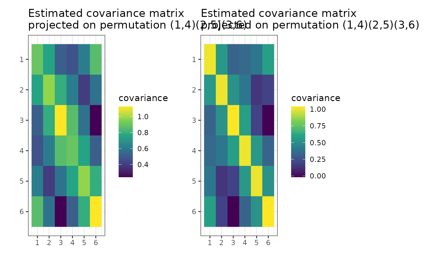# Now, the output is (most likely) different because the permutation
# `g_map[[1]]` is (most likely) not an identity permutation.

g_map_MH <- find_MAP(g, max_iter = 30, show_progress_bar = FALSE, optimizer = "MH")
if (require("graphics")) {
  plot(g_map_MH, type = "n0")
}

Plot optimized matrix or optimization `gipsmult` object

Usage

Arguments

Value

See also

Examples