The constructor of a gipsmult class.

Create a gipsmult object. This object will contain initial data and all other information needed to find the most likely invariant permutation. It will not perform optimization. One must call the find_MAP() function to do it. See the examples below.

Usage

gipsmult(
  Ss,
  numbers_of_observations,
  delta = 3,
  D_matrices = NULL,
  was_mean_estimated = TRUE,
  perm = ""
)

new_gipsmult(
  list_of_gips_perm,
  Ss,
  numbers_of_observations,
  delta,
  D_matrices,
  was_mean_estimated,
  optimization_info
)

Arguments

Ss

A list of matrices; empirical covariance matrices. When Z is the observed data from single class:

• if one does not know the theoretical mean and has to estimate it with the observed mean, use S = cov(Z), and leave parameter was_mean_estimated = TRUE as default;

• if one know the theoretical mean is 0, use S = (t(Z) %*% Z) / number_of_observations, and set parameter was_mean_estimated = FALSE.

numbers_of_observations

Numbers of data points that Ss is based on.

delta

A number, hyper-parameter of a Bayesian model. It has to be strictly bigger than 1. See the Hyperparameters section below.

D_matrices

A list of symmetric, positive-definite matrices of the same size as matrices in Ss. Hyper-parameter of a Bayesian model. When NULL, the (hopefully) reasonable one is derived from the data. For more details, see the Hyperparameters section below.

was_mean_estimated

A boolean.

• Set TRUE (default) when your S parameter is a result of a stats::cov() function.

• Set FALSE when your S parameter is a result of a (t(Z) %*% Z) / number_of_observations calculation.

perm

An optional permutation to be the base for the gipsmult object. It can be of a gips_perm or a permutation class, or anything the function permutations::permutation() can handle. It can also be of a gipsmult class, but it will be interpreted as the underlying gips_perm.

list_of_gips_perm

A list with a single element of a gips_perm class. The base object for the gipsmult object.

optimization_info

For internal use only. NULL or the list with information about the optimization process.

Value

gipsmult() returns an object of a gipsmult class after the safety checks.

new_gipsmult() returns an object of a gipsmult class without the safety checks.

Functions

• new_gipsmult(): Constructor. It is only intended for low-level use.

Methods for a gipsmult class

• plot.gipsmult()

• print.gipsmult()

Hyperparameters

We encourage the user to try D_matrix = d * I, where I is an identity matrix of a size p x p and d > 0 for some different d. When d is small compared to the data (e.g., d = 0.1 * mean(diag(S))), bigger structures will be found. When d is big compared to the data (e.g., d = 100 * mean(diag(S))), the posterior distribution does not depend on the data.

Taking D_matrix = d * I is equivalent to setting S <- S / d.

The default for D_matrix is D_matrix = d * I, where d = mean(diag(S)), which is equivalent to modifying S so that the mean value on the diagonal is 1.

In the Bayesian model, the prior distribution for the covariance matrix is a generalized case of Wishart distribution.

See also

• stats::cov() – The Ss parameter, as a list of empirical covariance matrices, is most of the time a result of the cov() function. For more information, see Wikipedia - Estimation of covariance matrices.

• find_MAP() – The function that finds the Maximum A Posteriori (MAP) Estimator for a given gipsmult object.

• gips::gips_perm() – The constructor of a gips_perm class. The gips_perm object is used as the base object for the gipsmult object.

Examples

perm_size <- 5
numbers_of_observations <- c(15, 18, 19)
Sigma <- diag(rep(1, perm_size))
n_matrices <- 3
df <- 20
Ss <- rWishart(n = n_matrices, df = df, Sigma = Sigma)
Ss <- lapply(1:n_matrices, function(x) Ss[, , x])
g <- gipsmult(Ss, numbers_of_observations)

g_map <- find_MAP(g, show_progress_bar = FALSE, optimizer = "brute_force")
g_map
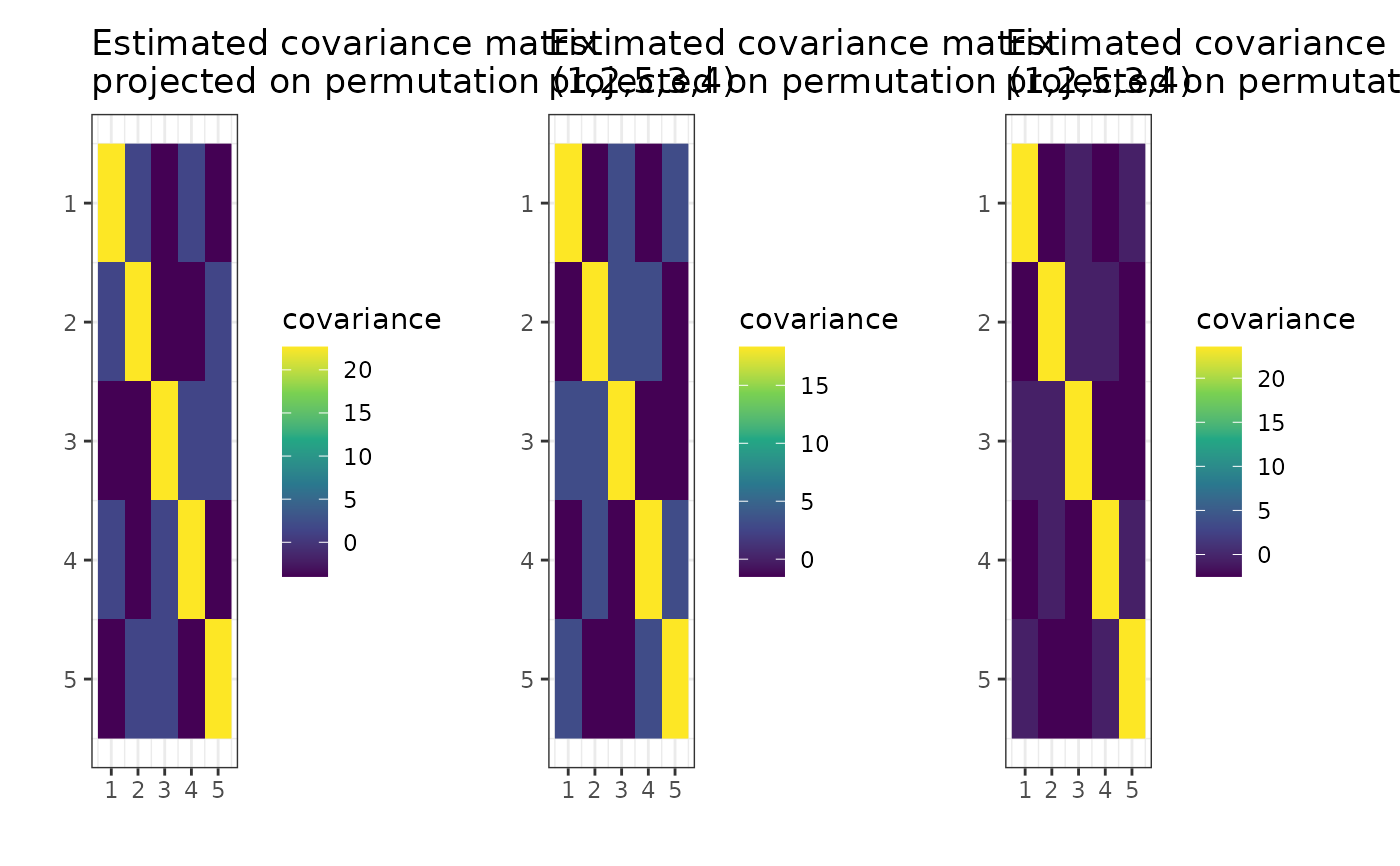
#> The permutation (1,2,5,3,4):
#>  - was found after 67 posteriori calculations;
#>  - is 1.132e+22 times more likely than the () permutation.

print(g_map)
#> The permutation (1,2,5,3,4):
#>  - was found after 67 posteriori calculations;
#>  - is 1.132e+22 times more likely than the () permutation.

if (require("graphics")) {
  plot(g_map, type = "MLE", logarithmic_x = TRUE)
}