Getting started with gipsDA • gipsDA

Overview

gipsDA extends classical Linear Discriminant Analysis (LDA) and Quadratic Discriminant Analysis (QDA) by replacing standard empirical covariance estimates with covariance estimates regularized by permutation-invariant structures learned with the gips framework.

The package provides three model-fitting functions:

gipslda() - LDA with a projected pooled covariance matrix.
gipsqda() - QDA with independently projected class-specific covariance matrices.
gipsmultqda() - QDA with class-specific covariance matrices and a jointly estimated permutation structure.

The functions follow the familiar conventions of MASS::lda() and MASS::qda(): they support formula, matrix, and data-frame interfaces, and their predict() methods return predicted classes and posterior probabilities.

Installation

Install the released version from CRAN:

install.packages("gipsDA")

Or install the development version from GitHub:

pak::pkg_install("AntoniKingston/gipsDA")

Load the package:

library(gipsDA)

Quick start

We use the built-in iris data set and create a simple stratified train/test split.

set.seed(42)

train_id <- unlist(
  lapply(split(seq_len(nrow(iris)), iris$Species), sample, size = 35),
  use.names = FALSE
)

train <- iris[train_id, ]
test <- iris[-train_id, ]

Fit a gipslda() model using the formula interface.

fit <- gipslda(Species ~ ., data = train)

fit
#> Call:
#> gipslda(Species ~ ., data = train)
#> 
#> Model: gipslda 
#> Number of observations: 105 
#> Number of groups: 3 
#> Number of predictors: 4 
#> 
#> Fitting options:
#> $MAP
#> [1] TRUE
#> 
#> $optimizer
#> [1] "BF"
#> 
#> $max_iter
#> NULL
#> 
#> $weighted_avg
#> [1] FALSE
#> 
#> $store_probabilities
#> [1] TRUE
#> 
#> 
#> Prior probabilities of groups:
#>     setosa versicolor  virginica 
#>  0.3333333  0.3333333  0.3333333 
#> 
#> Class counts:
#>     setosa versicolor  virginica 
#>         35         35         35 
#> 
#> Group means:
#>            Sepal.Length Sepal.Width Petal.Length Petal.Width
#> setosa         5.020000    3.420000     1.482857   0.2428571
#> versicolor     5.911429    2.771429     4.302857   1.3371429
#> virginica      6.725714    3.020000     5.654286   2.0685714
#> 
#> Selected MAP permutation: (1,2,4,3) 
#> 
#> Posterior probabilities of retained permutations:
#>   (1,2,4,3)  (1,3)(2,4)   (1,2,3,4)  (1,2)(3,4)  (1,4)(2,3) 
#> 0.549732245 0.423533797 0.018304175 0.004073983 0.003658725 
#> 
#> Coefficients of linear discriminants:
#>                     LD1        LD2
#> Sepal.Length -0.2534381 -0.3641984
#> Sepal.Width   2.3946991 -2.3105323
#> Petal.Length -1.3688435  0.8934580
#> Petal.Width  -3.5168812 -2.3906963
#> 
#> Proportion of trace:
#>    LD1    LD2 
#> 0.9888 0.0112

Predict classes for the test set.

pred <- predict(fit, test)

head(pred$class)
#> [1] setosa setosa setosa setosa setosa setosa
#> Levels: setosa versicolor virginica
head(pred$posterior)
#>    setosa   versicolor    virginica
#> 6       1 4.955555e-22 1.956129e-41
#> 9       1 1.894514e-16 8.017336e-36
#> 14      1 8.720623e-21 8.034755e-42
#> 16      1 1.868380e-28 2.037539e-49
#> 17      1 1.869751e-24 1.343241e-44
#> 19      1 5.185944e-22 1.062783e-41

mean(pred$class == test$Species)
#> [1] 0.9777778

Preparing data

gipsDA works with numeric predictors and a categorical grouping variable.

Before fitting a model:

remove or impute missing values,
remove non-informative columns, such as identifiers,
encode categorical predictors before passing them to the model,
avoid mixing variables with incomparable scales when possible.

Because the method searches for symmetries between variables, predictors should be meaningfully comparable. For example, variables measured in the same units or representing analogous sensor readings are more natural candidates for permutation symmetry.

Standardization can be useful when predictors are on very different scales, but it should be done carefully. In particular, scaling parameters should be estimated on the training data only and then applied to new data.

Model relationships

The three gipsDA models are related to classical LDA and QDA as shown below.

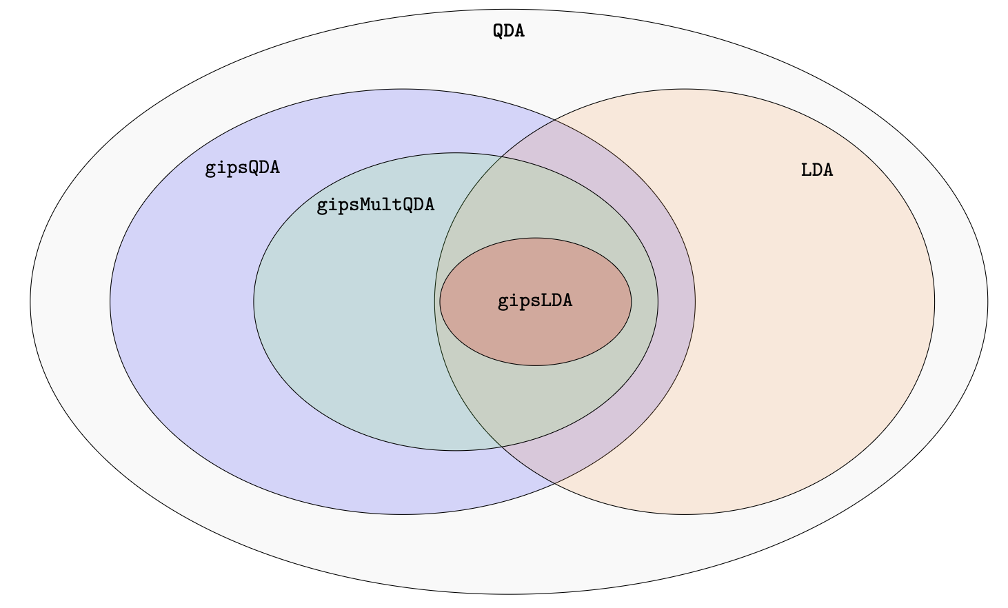
The diagram illustrates the hierarchical relationships between the models.

The figure illustrates the inclusion relations between the model classes. gipsqda() is contained in QDA, gipslda() is contained in LDA, and gipsmultqda() lies between gipsqda() and gipslda().

Choosing a model

Function	Covariance-matrix assumption	When this may be reasonable
`gipslda()`	all classes share one projected covariance matrix	classes differ mainly in their means, but have similar covariance structure
`gipsqda()`	each class has its own projected covariance matrix and its own permutation structure	classes may have different covariance patterns
`gipsmultqda()`	each class has its own covariance matrix, but all classes share one permutation structure	classes differ in scale or variance, but have a common dependency pattern between features

Key arguments

Argument	Meaning
`prior`	prior probabilities of classes
`MAP`	whether to use the Maximum A Posteriori permutation or posterior-weighted averaging
`optimizer`	permutation-search strategy: `"BF"` or `"MH"`
`max_iter`	number of Metropolis-Hastings iterations when `optimizer = "MH"`
`weighted_avg`	covariance pooling strategy for `gipslda()`
`tol`	numerical tolerance used during fitting

MAP: Maximum A Posteriori

When MAP = TRUE, the model selects the single most probable permutation structure and uses the covariance matrix projected onto that structure.

lda_map <- gipslda(
  Species ~ .,
  data = train,
  MAP = TRUE
)

lda_map
#> Call:
#> gipslda(Species ~ ., data = train, MAP = TRUE)
#> 
#> Model: gipslda 
#> Number of observations: 105 
#> Number of groups: 3 
#> Number of predictors: 4 
#> 
#> Fitting options:
#> $MAP
#> [1] TRUE
#> 
#> $optimizer
#> [1] "BF"
#> 
#> $max_iter
#> NULL
#> 
#> $weighted_avg
#> [1] FALSE
#> 
#> $store_probabilities
#> [1] TRUE
#> 
#> 
#> Prior probabilities of groups:
#>     setosa versicolor  virginica 
#>  0.3333333  0.3333333  0.3333333 
#> 
#> Class counts:
#>     setosa versicolor  virginica 
#>         35         35         35 
#> 
#> Group means:
#>            Sepal.Length Sepal.Width Petal.Length Petal.Width
#> setosa         5.020000    3.420000     1.482857   0.2428571
#> versicolor     5.911429    2.771429     4.302857   1.3371429
#> virginica      6.725714    3.020000     5.654286   2.0685714
#> 
#> Selected MAP permutation: (1,2,4,3) 
#> 
#> Posterior probabilities of retained permutations:
#>   (1,2,4,3)  (1,3)(2,4)   (1,2,3,4)  (1,2)(3,4)  (1,4)(2,3) 
#> 0.549732245 0.423533797 0.018304175 0.004073983 0.003658725 
#> 
#> Coefficients of linear discriminants:
#>                     LD1        LD2
#> Sepal.Length -0.2534381 -0.3641984
#> Sepal.Width   2.3946991 -2.3105323
#> Petal.Length -1.3688435  0.8934580
#> Petal.Width  -3.5168812 -2.3906963
#> 
#> Proportion of trace:
#>    LD1    LD2 
#> 0.9888 0.0112

When MAP = FALSE, the model uses posterior probabilities over retained permutation structures and computes a posterior-weighted covariance estimate.

lda_avg <- gipslda(
  Species ~ .,
  data = train,
  MAP = FALSE
)

lda_avg
#> Call:
#> gipslda(Species ~ ., data = train, MAP = FALSE)
#> 
#> Model: gipslda 
#> Number of observations: 105 
#> Number of groups: 3 
#> Number of predictors: 4 
#> 
#> Fitting options:
#> $MAP
#> [1] FALSE
#> 
#> $optimizer
#> [1] "BF"
#> 
#> $max_iter
#> NULL
#> 
#> $weighted_avg
#> [1] FALSE
#> 
#> $store_probabilities
#> [1] TRUE
#> 
#> 
#> Prior probabilities of groups:
#>     setosa versicolor  virginica 
#>  0.3333333  0.3333333  0.3333333 
#> 
#> Class counts:
#>     setosa versicolor  virginica 
#>         35         35         35 
#> 
#> Group means:
#>            Sepal.Length Sepal.Width Petal.Length Petal.Width
#> setosa         5.020000    3.420000     1.482857   0.2428571
#> versicolor     5.911429    2.771429     4.302857   1.3371429
#> virginica      6.725714    3.020000     5.654286   2.0685714
#> 
#> Posterior probabilities of retained permutations:
#>   (1,2,4,3)  (1,3)(2,4)   (1,2,3,4)  (1,2)(3,4)  (1,4)(2,3) 
#> 0.549732245 0.423533797 0.018304175 0.004073983 0.003658725 
#> 
#> Coefficients of linear discriminants:
#>                      LD1        LD2
#> Sepal.Length  0.06710214 -0.5349658
#> Sepal.Width   2.15454818 -2.2243646
#> Petal.Length -1.59385584  0.9770055
#> Petal.Width  -3.36967333 -2.4060085
#> 
#> Proportion of trace:
#>    LD1    LD2 
#> 0.9886 0.0114

In printed model output, a result such as (1243) is written in cycle notation. It means that the permutation maps feature 1 to 2, 2 to 4, 4 to 3, and 3 back to 1. Features appearing in the same cycle are treated as exchangeable under the selected symmetry structure.

For formulas and a more detailed explanation of posterior averaging, see the Advanced usage vignette.

Optimizer

The optimizer argument controls how permutation structures are searched.

Value	Meaning	Recommended use
`"BF"`	brute-force search	small number of dimensions, default for `p <= 10`
`"MH"`	Metropolis-Hastings search	larger number of dimensions, default for `p > 10`

For optimizer = "MH", use max_iter to control the number of iterations.

fit_mh <- gipsqda(
  Species ~ .,
  data = train,
  optimizer = "MH",
  max_iter = 1000
)

For optimizer = "BF", max_iter is ignored.

For more details about optimization settings, see the Advanced usage vignette.

Fitting all three models

lda_fit <- gipslda(Species ~ ., data = train)
qda_fit <- gipsqda(Species ~ ., data = train)
joint_qda_fit <- gipsmultqda(Species ~ ., data = train)

lda_pred <- predict(lda_fit, test)
qda_pred <- predict(qda_fit, test)
joint_qda_pred <- predict(joint_qda_fit, test)

c(
  gipslda = mean(lda_pred$class == test$Species),
  gipsqda = mean(qda_pred$class == test$Species),
  gipsmultqda = mean(joint_qda_pred$class == test$Species)
)
#>     gipslda     gipsqda gipsmultqda 
#>   0.9777778   0.9777778   1.0000000

Inspecting a fitted model

The most readable way to inspect a fitted model is to print it.

print(lda_fit)
#> Call:
#> gipslda(Species ~ ., data = train)
#> 
#> Model: gipslda 
#> Number of observations: 105 
#> Number of groups: 3 
#> Number of predictors: 4 
#> 
#> Fitting options:
#> $MAP
#> [1] TRUE
#> 
#> $optimizer
#> [1] "BF"
#> 
#> $max_iter
#> NULL
#> 
#> $weighted_avg
#> [1] FALSE
#> 
#> $store_probabilities
#> [1] TRUE
#> 
#> 
#> Prior probabilities of groups:
#>     setosa versicolor  virginica 
#>  0.3333333  0.3333333  0.3333333 
#> 
#> Class counts:
#>     setosa versicolor  virginica 
#>         35         35         35 
#> 
#> Group means:
#>            Sepal.Length Sepal.Width Petal.Length Petal.Width
#> setosa         5.020000    3.420000     1.482857   0.2428571
#> versicolor     5.911429    2.771429     4.302857   1.3371429
#> virginica      6.725714    3.020000     5.654286   2.0685714
#> 
#> Selected MAP permutation: (1,2,4,3) 
#> 
#> Posterior probabilities of retained permutations:
#>   (1,2,4,3)  (1,3)(2,4)   (1,2,3,4)  (1,2)(3,4)  (1,4)(2,3) 
#> 0.549732245 0.423533797 0.018304175 0.004073983 0.003658725 
#> 
#> Coefficients of linear discriminants:
#>                     LD1        LD2
#> Sepal.Length -0.2534381 -0.3641984
#> Sepal.Width   2.3946991 -2.3105323
#> Petal.Length -1.3688435  0.8934580
#> Petal.Width  -3.5168812 -2.3906963
#> 
#> Proportion of trace:
#>    LD1    LD2 
#> 0.9888 0.0112

The printed output shows the model call, class priors, group means, and information about selected or averaged permutation structures.

If a dedicated summary() method is available, it can be used for a more compact model summary.

summary(lda_fit)
#> Call:
#> gipslda(Species ~ ., data = train)
#> 
#> Model: gipslda 
#> Number of observations: 105 
#> Number of groups: 3 
#> Number of predictors: 4 
#> 
#> Fitting options:
#> $MAP
#> [1] TRUE
#> 
#> $optimizer
#> [1] "BF"
#> 
#> $max_iter
#> NULL
#> 
#> $weighted_avg
#> [1] FALSE
#> 
#> $store_probabilities
#> [1] TRUE
#> 
#> 
#> Class counts:
#>     setosa versicolor  virginica 
#>         35         35         35 
#> 
#> Prior probabilities of groups:
#>     setosa versicolor  virginica 
#>  0.3333333  0.3333333  0.3333333 
#> 
#> Group means:
#>            Sepal.Length Sepal.Width Petal.Length Petal.Width
#> setosa         5.020000    3.420000     1.482857   0.2428571
#> versicolor     5.911429    2.771429     4.302857   1.3371429
#> virginica      6.725714    3.020000     5.654286   2.0685714
#> 
#> Proportion of trace:
#>    LD1    LD2 
#> 0.9888 0.0112 
#> 
#> Selected MAP permutation: (1,2,4,3) 
#> 
#> Posterior probabilities of retained permutations:
#>   (1,2,4,3)  (1,3)(2,4)   (1,2,3,4)  (1,2)(3,4)  (1,4)(2,3) 
#> 0.549732245 0.423533797 0.018304175 0.004073983 0.003658725

More details about fitted model objects are described in the Advanced usage vignette.

Prediction output

Prediction returns predicted classes and posterior probabilities.

head(lda_pred$class)
#> [1] setosa setosa setosa setosa setosa setosa
#> Levels: setosa versicolor virginica
head(lda_pred$posterior)
#>    setosa   versicolor    virginica
#> 6       1 4.955555e-22 1.956129e-41
#> 9       1 1.894514e-16 8.017336e-36
#> 14      1 8.720623e-21 8.034755e-42
#> 16      1 1.868380e-28 2.037539e-49
#> 17      1 1.869751e-24 1.343241e-44
#> 19      1 5.185944e-22 1.062783e-41

More detailed prediction options are described in the Advanced usage vignette.

Matrix interface

The formula interface is usually the most convenient, but the matrix interface is also available.

x <- as.matrix(iris[, 1:4])
grouping <- iris$Species

fit_matrix <- gipslda(x, grouping)

predict(fit_matrix, x[1:5, ])$class
#> [1] setosa setosa setosa setosa setosa
#> Levels: setosa versicolor virginica

The same style can be used with gipsqda() and gipsmultqda().

qda_matrix <- gipsqda(x, grouping)
joint_qda_matrix <- gipsmultqda(x, grouping)

predict(qda_matrix, x[1:5, ])$class
#> [1] setosa setosa setosa setosa setosa
#> Levels: setosa versicolor virginica
predict(joint_qda_matrix, x[1:5, ])$class
#> [1] setosa setosa setosa setosa setosa
#> Levels: setosa versicolor virginica

Summary

For a first analysis, start with:

fit <- gipslda(Species ~ ., data = train)
pred <- predict(fit, test)

mean(pred$class == test$Species)
#> [1] 0.9777778

Use:

Function	Use when
`gipslda()`	classes can reasonably share one covariance structure
`gipsqda()`	each class may have its own covariance structure
`gipsmultqda()`	classes may have different covariance matrices but a shared dependency pattern

The main tuning choices are:

Argument	Practical meaning
`MAP = TRUE`	use one selected Maximum A Posteriori permutation
`MAP = FALSE`	average over retained permutations using posterior probabilities
`optimizer = "BF"`	exhaustive search, default for `p <= 10`
`optimizer = "MH"`	stochastic search, default for `p > 10`
`max_iter`	used only with `optimizer = "MH"`
`weighted_avg`	changes the pooled covariance estimator in `gipslda()`
`store_probabilities`	whether to store posterior probabilities of retained permutations

More detailed examples, including weighted_avg, leave-one-out prediction, matrix interfaces, and model diagnostics, are described in the Advanced usage vignette.