Advanced usage of gipsDA

Overview

This vignette gives a more detailed overview of the main modeling options in gipsDA.

It covers:

data preparation,
the differences between gipslda(), gipsqda(), and gipsmultqda(),
the MAP, optimizer, max_iter, prior, and weighted_avg arguments,
interpretation of permutation output,
prediction methods,
leave-one-out prediction,
model inspection and diagnostics.

For a shorter first example, see the Getting started vignette.

library(gipsDA)

Example data

We use the built-in iris data set.

set.seed(42)

train_id <- unlist(
  lapply(split(seq_len(nrow(iris)), iris$Species), sample, size = 35),
  use.names = FALSE
)

train <- iris[train_id, ]
test <- iris[-train_id, ]

table(train$Species)
#> 
#>     setosa versicolor  virginica 
#>         35         35         35
table(test$Species)
#> 
#>     setosa versicolor  virginica 
#>         15         15         15

Preparing data

gipsDA models assume numeric predictors and a categorical grouping variable.

Before fitting a model, it is usually useful to:

remove identifier columns,
remove or impute missing values,
remove constant or almost constant columns,
encode categorical predictors,
check whether predictors are on comparable scales.

The last point is especially important for gipsDA. The method searches for permutation symmetries between variables. Such symmetries are most meaningful when variables are comparable, for example when they are measured in the same units or represent analogous sensor readings.

Checking predictor types

str(train)
#> 'data.frame':    105 obs. of  5 variables:
#>  $ Sepal.Length: num  5.3 5.5 5.1 4.8 4.9 5 5.1 5.1 4.6 5.1 ...
#>  $ Sepal.Width : num  3.7 3.5 3.5 3.4 3.1 3.2 3.5 3.3 3.4 3.8 ...
#>  $ Petal.Length: num  1.5 1.3 1.4 1.9 1.5 1.2 1.4 1.7 1.4 1.9 ...
#>  $ Petal.Width : num  0.2 0.2 0.2 0.2 0.1 0.2 0.3 0.5 0.3 0.4 ...
#>  $ Species     : Factor w/ 3 levels "setosa","versicolor",..: 1 1 1 1 1 1 1 1 1 1 ...

For formula-based usage, the response variable should be a factor or a categorical variable.

is.factor(train$Species)
#> [1] TRUE

The predictors in iris are already numeric.

vapply(train[, 1:4], is.numeric, logical(1))
#> Sepal.Length  Sepal.Width Petal.Length  Petal.Width 
#>         TRUE         TRUE         TRUE         TRUE

Scaling predictors

Scaling may be useful when predictors are measured on very different scales. However, scaling should be done carefully: the center and scale should be estimated only on the training data and then applied to new data.

x_train <- train[, 1:4]
x_test <- test[, 1:4]

train_center <- vapply(x_train, mean, numeric(1))
train_scale <- vapply(x_train, sd, numeric(1))

train_scaled <- train
test_scaled <- test

train_scaled[, 1:4] <- scale(
  x_train,
  center = train_center,
  scale = train_scale
)

test_scaled[, 1:4] <- scale(
  x_test,
  center = train_center,
  scale = train_scale
)

Then fit the model on the scaled data.

fit_scaled <- gipslda(Species ~ ., data = train_scaled)
pred_scaled <- predict(fit_scaled, test_scaled)

mean(pred_scaled$class == test_scaled$Species)
#> [1] 0.9777778

Scaling is not always necessary. It depends on whether the original variables are already comparable and whether scaling is meaningful for the application.

Model choice

The package provides three main classifiers.

Function	Covariance-matrix assumption	Typical use case
`gipslda()`	all classes share one projected covariance matrix	classes differ mainly in their means
`gipsqda()`	each class has its own projected covariance matrix and its own permutation structure	classes may have different covariance patterns
`gipsmultqda()`	each class has its own covariance matrix, but all classes share one permutation structure	classes may differ in scale, but share a dependency pattern

Fit all three models on the same data.

lda_fit <- gipslda(Species ~ ., data = train)
qda_fit <- gipsqda(Species ~ ., data = train)
joint_qda_fit <- gipsmultqda(Species ~ ., data = train)

Compare test-set accuracy.

lda_pred <- predict(lda_fit, test)
qda_pred <- predict(qda_fit, test)
joint_qda_pred <- predict(joint_qda_fit, test)

c(
  gipslda = mean(lda_pred$class == test$Species),
  gipsqda = mean(qda_pred$class == test$Species),
  gipsmultqda = mean(joint_qda_pred$class == test$Species)
)
#>     gipslda     gipsqda gipsmultqda 
#>   0.9777778   0.9777778   1.0000000

Model hierarchy

The inclusion relations between the model classes are shown below.

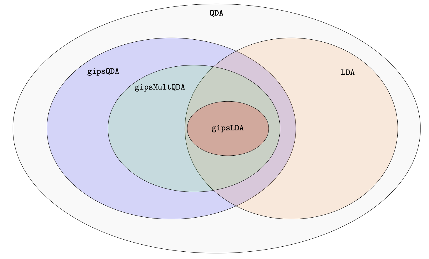
The diagram illustrates the hierarchical relationships between the models.

The figure shows that gipsqda() is contained in QDA, gipslda() is contained in LDA, and gipsmultqda() lies between gipsqda() and gipslda().

In practical terms, moving inward in the diagram means imposing stronger assumptions on the covariance structure. Stronger assumptions can reduce estimation variance, especially when the number of observations is small, but they may be too restrictive if the assumed structure is not present in the data.

MAP: Maximum A Posteriori

MAP stands for Maximum A Posteriori.

The MAP argument controls how the covariance matrix is projected after the permutation search.

When MAP = TRUE, the model selects the single most probable permutation structure and projects the covariance matrix onto the invariant space determined by that structure.

lda_map <- gipslda(
  Species ~ .,
  data = train,
  MAP = TRUE
)

lda_map
#> Call:
#> gipslda(Species ~ ., data = train, MAP = TRUE)
#> 
#> Model: gipslda 
#> Number of observations: 105 
#> Number of groups: 3 
#> Number of predictors: 4 
#> 
#> Fitting options:
#> $MAP
#> [1] TRUE
#> 
#> $optimizer
#> [1] "BF"
#> 
#> $max_iter
#> NULL
#> 
#> $weighted_avg
#> [1] FALSE
#> 
#> $store_probabilities
#> [1] TRUE
#> 
#> 
#> Prior probabilities of groups:
#>     setosa versicolor  virginica 
#>  0.3333333  0.3333333  0.3333333 
#> 
#> Class counts:
#>     setosa versicolor  virginica 
#>         35         35         35 
#> 
#> Group means:
#>            Sepal.Length Sepal.Width Petal.Length Petal.Width
#> setosa         5.020000    3.420000     1.482857   0.2428571
#> versicolor     5.911429    2.771429     4.302857   1.3371429
#> virginica      6.725714    3.020000     5.654286   2.0685714
#> 
#> Selected MAP permutation: (1,2,4,3) 
#> 
#> Posterior probabilities of retained permutations:
#>   (1,2,4,3)  (1,3)(2,4)   (1,2,3,4)  (1,2)(3,4)  (1,4)(2,3) 
#> 0.549732245 0.423533797 0.018304175 0.004073983 0.003658725 
#> 
#> Coefficients of linear discriminants:
#>                     LD1        LD2
#> Sepal.Length -0.2534381 -0.3641984
#> Sepal.Width   2.3946991 -2.3105323
#> Petal.Length -1.3688435  0.8934580
#> Petal.Width  -3.5168812 -2.3906963
#> 
#> Proportion of trace:
#>    LD1    LD2 
#> 0.9888 0.0112

When MAP = FALSE, the model uses posterior probabilities over retained permutation structures and computes a posterior-weighted projection.

lda_avg <- gipslda(
  Species ~ .,
  data = train,
  MAP = FALSE
)

lda_avg
#> Call:
#> gipslda(Species ~ ., data = train, MAP = FALSE)
#> 
#> Model: gipslda 
#> Number of observations: 105 
#> Number of groups: 3 
#> Number of predictors: 4 
#> 
#> Fitting options:
#> $MAP
#> [1] FALSE
#> 
#> $optimizer
#> [1] "BF"
#> 
#> $max_iter
#> NULL
#> 
#> $weighted_avg
#> [1] FALSE
#> 
#> $store_probabilities
#> [1] TRUE
#> 
#> 
#> Prior probabilities of groups:
#>     setosa versicolor  virginica 
#>  0.3333333  0.3333333  0.3333333 
#> 
#> Class counts:
#>     setosa versicolor  virginica 
#>         35         35         35 
#> 
#> Group means:
#>            Sepal.Length Sepal.Width Petal.Length Petal.Width
#> setosa         5.020000    3.420000     1.482857   0.2428571
#> versicolor     5.911429    2.771429     4.302857   1.3371429
#> virginica      6.725714    3.020000     5.654286   2.0685714
#> 
#> Posterior probabilities of retained permutations:
#>   (1,2,4,3)  (1,3)(2,4)   (1,2,3,4)  (1,2)(3,4)  (1,4)(2,3) 
#> 0.549732245 0.423533797 0.018304175 0.004073983 0.003658725 
#> 
#> Coefficients of linear discriminants:
#>                      LD1        LD2
#> Sepal.Length  0.06710214 -0.5349658
#> Sepal.Width   2.15454818 -2.2243646
#> Petal.Length -1.59385584  0.9770055
#> Petal.Width  -3.36967333 -2.4060085
#> 
#> Proportion of trace:
#>    LD1    LD2 
#> 0.9886 0.0114

Conceptually, if $S$ is an empirical covariance matrix and $S_c$ is its projection under permutation structure $c$ , then the two approaches can be summarized as follows.

For MAP = TRUE:

$\hat{S} = S_{c^*},$

where

$c^* = \arg\max_c P(c \mid X).$

For MAP = FALSE:

$\hat{S} = \sum_c P(c \mid X) S_c.$

The second option averages over several possible symmetry structures instead of using only one selected structure.

By default, gipsDA stores posterior probabilities of retained permutations. For faster MAP-only fitting, set store_probabilities = FALSE. In that case, the selected MAP permutation is still stored and shown, but posterior probabilities are not stored in the fitted model object.

Interpreting permutation output

Printed model output may contain permutations such as:

(1,2)
(1,2)(3,4)
(1,2,4,3)
()

This notation is called cycle notation.

For example, the cycle

(1,2,4,3)

means that the permutation maps:

1 -> 2
2 -> 4
4 -> 3
3 -> 1

A product of cycles such as:

(1,2)(3,4)

means that feature 1 is swapped with feature 2, and feature 3 is swapped with feature 4.

The empty permutation:

()

is the identity permutation. It means that no non-trivial permutation symmetry was selected.

In the context of gipsDA, a selected permutation structure describes which features are treated as exchangeable by the covariance model.

Optimizer

The optimizer argument controls how permutation structures are searched.

Value	Meaning	Typical use
`"BF"`	brute-force search	small number of dimensions, default for `p <= 10`
`"MH"`	Metropolis-Hastings search	larger number of dimensions, default for `p > 10`

The brute-force optimizer searches the relevant permutation space exhaustively. It is deterministic, but its cost grows quickly with the number of features.

fit_bf <- gipsqda(
  Species ~ .,
  data = train,
  optimizer = "BF"
)

fit_bf
#> Call:
#> gipsqda(Species ~ ., data = train, optimizer = "BF")
#> 
#> Model: gipsqda 
#> Number of observations: 105 
#> Number of groups: 3 
#> Number of predictors: 4 
#> 
#> Fitting options:
#> $MAP
#> [1] TRUE
#> 
#> $optimizer
#> [1] "BF"
#> 
#> $max_iter
#> NULL
#> 
#> $store_probabilities
#> [1] TRUE
#> 
#> 
#> Prior probabilities of groups:
#>     setosa versicolor  virginica 
#>  0.3333333  0.3333333  0.3333333 
#> 
#> Class counts:
#>     setosa versicolor  virginica 
#>         35         35         35 
#> 
#> Group means:
#>            Sepal.Length Sepal.Width Petal.Length Petal.Width
#> setosa         5.020000    3.420000     1.482857   0.2428571
#> versicolor     5.911429    2.771429     4.302857   1.3371429
#> virginica      6.725714    3.020000     5.654286   2.0685714
#> 
#> Group: setosa 
#> Selected MAP permutation: (1,2) 
#> 
#> Group: versicolor 
#> Selected MAP permutation: (2,3) 
#> 
#> Group: virginica 
#> Selected MAP permutation: (1,3)(2,4) 
#> 
#> Posterior probabilities of retained permutations:
#> 
#> Group: setosa 
#>       (1,2)  (1,2)(3,4)       (3,4)          () 
#> 0.562114561 0.404501310 0.024221480 0.008570546 
#> 
#> Group: versicolor 
#>       (2,3)          ()       (1,3)     (1,2,3)       (1,2)  (1,3)(2,4) 
#> 0.889698934 0.061618087 0.029058419 0.015073718 0.002647551 0.001632264 
#> 
#> Group: virginica 
#>  (1,3)(2,4)       (1,3)       (2,4)          () 
#> 0.849678403 0.089183371 0.058826178 0.001555686 
#> 
#> Log determinants of projected covariance matrices:
#> [1] -10.197338  -8.531728  -8.239145

For larger problems, use the Metropolis-Hastings optimizer.

fit_mh <- gipsqda(
  Species ~ .,
  data = train,
  optimizer = "MH",
  max_iter = 1000
)

`max_iter`

max_iter controls the number of Metropolis-Hastings iterations when optimizer = "MH".

Increasing max_iter gives the stochastic search more time to explore the permutation space, but also increases runtime.

fit_mh_100 <- gipsqda(
  Species ~ .,
  data = train,
  optimizer = "MH",
  max_iter = 100
)

fit_mh_1000 <- gipsqda(
  Species ~ .,
  data = train,
  optimizer = "MH",
  max_iter = 1000
)

For optimizer = "BF", max_iter is ignored.

Class priors

The prior argument specifies prior probabilities of classes.

By default, priors are estimated from the training data.

lda_fit$prior
#>     setosa versicolor  virginica 
#>  0.3333333  0.3333333  0.3333333

You can set them manually.

equal_prior <- rep(1 / length(levels(train$Species)), length(levels(train$Species)))
names(equal_prior) <- levels(train$Species)

lda_equal_prior <- gipslda(
  Species ~ .,
  data = train,
  prior = equal_prior
)

lda_equal_prior$prior
#>     setosa versicolor  virginica 
#>  0.3333333  0.3333333  0.3333333

The prior vector should contain one value per class and should sum to one.

sum(equal_prior)
#> [1] 1

Class priors affect posterior probabilities and may affect predicted classes, especially when classes overlap.

`weighted_avg` in `gipslda()`

The weighted_avg argument is specific to gipslda().

It controls how the pooled covariance matrix is constructed before the gips projection is applied.

Let:

$K$ be the number of classes,
$n_k$ be the number of observations in class $k$ ,
$n = \sum_{k=1}^{K} n_k$ be the total number of observations,
$S_k$ be the sample covariance matrix in class $k$ .

With weighted_avg = FALSE, gipslda() uses the classic pooled covariance estimator:

$S_{\mathrm{classic}} = \frac{1}{n - K} \sum_{k = 1}^{K} (n_k - 1) S_k.$

With weighted_avg = TRUE, gipslda() uses:

$S_{\mathrm{weighted}} = \frac{1}{n} \sum_{k = 1}^{K} n_k S_k.$

Fit both variants.

lda_classic <- gipslda(
  Species ~ .,
  data = train,
  weighted_avg = FALSE
)

lda_weighted <- gipslda(
  Species ~ .,
  data = train,
  weighted_avg = TRUE
)

Compare predictions.

pred_classic <- predict(lda_classic, test)
pred_weighted <- predict(lda_weighted, test)

c(
  classic = mean(pred_classic$class == test$Species),
  weighted = mean(pred_weighted$class == test$Species)
)
#>   classic  weighted 
#> 0.9777778 0.9777778

The two variants can behave differently when class sizes are imbalanced or when class-specific covariance estimates differ substantially.

Formula interface

The formula interface is usually the most convenient interface.

fit_formula <- gipslda(
  Species ~ Sepal.Length + Sepal.Width + Petal.Length + Petal.Width,
  data = train
)

fit_formula
#> Call:
#> gipslda(Species ~ Sepal.Length + Sepal.Width + Petal.Length + 
#>     Petal.Width, data = train)
#> 
#> Model: gipslda 
#> Number of observations: 105 
#> Number of groups: 3 
#> Number of predictors: 4 
#> 
#> Fitting options:
#> $MAP
#> [1] TRUE
#> 
#> $optimizer
#> [1] "BF"
#> 
#> $max_iter
#> NULL
#> 
#> $weighted_avg
#> [1] FALSE
#> 
#> $store_probabilities
#> [1] TRUE
#> 
#> 
#> Prior probabilities of groups:
#>     setosa versicolor  virginica 
#>  0.3333333  0.3333333  0.3333333 
#> 
#> Class counts:
#>     setosa versicolor  virginica 
#>         35         35         35 
#> 
#> Group means:
#>            Sepal.Length Sepal.Width Petal.Length Petal.Width
#> setosa         5.020000    3.420000     1.482857   0.2428571
#> versicolor     5.911429    2.771429     4.302857   1.3371429
#> virginica      6.725714    3.020000     5.654286   2.0685714
#> 
#> Selected MAP permutation: (1,2,4,3) 
#> 
#> Posterior probabilities of retained permutations:
#>   (1,2,4,3)  (1,3)(2,4)   (1,2,3,4)  (1,2)(3,4)  (1,4)(2,3) 
#> 0.549732245 0.423533797 0.018304175 0.004073983 0.003658725 
#> 
#> Coefficients of linear discriminants:
#>                     LD1        LD2
#> Sepal.Length -0.2534381 -0.3641984
#> Sepal.Width   2.3946991 -2.3105323
#> Petal.Length -1.3688435  0.8934580
#> Petal.Width  -3.5168812 -2.3906963
#> 
#> Proportion of trace:
#>    LD1    LD2 
#> 0.9888 0.0112

The shorthand Species ~ . uses all remaining columns as predictors.

fit_formula_short <- gipslda(
  Species ~ .,
  data = train
)

fit_formula_short
#> Call:
#> gipslda(Species ~ ., data = train)
#> 
#> Model: gipslda 
#> Number of observations: 105 
#> Number of groups: 3 
#> Number of predictors: 4 
#> 
#> Fitting options:
#> $MAP
#> [1] TRUE
#> 
#> $optimizer
#> [1] "BF"
#> 
#> $max_iter
#> NULL
#> 
#> $weighted_avg
#> [1] FALSE
#> 
#> $store_probabilities
#> [1] TRUE
#> 
#> 
#> Prior probabilities of groups:
#>     setosa versicolor  virginica 
#>  0.3333333  0.3333333  0.3333333 
#> 
#> Class counts:
#>     setosa versicolor  virginica 
#>         35         35         35 
#> 
#> Group means:
#>            Sepal.Length Sepal.Width Petal.Length Petal.Width
#> setosa         5.020000    3.420000     1.482857   0.2428571
#> versicolor     5.911429    2.771429     4.302857   1.3371429
#> virginica      6.725714    3.020000     5.654286   2.0685714
#> 
#> Selected MAP permutation: (1,2,4,3) 
#> 
#> Posterior probabilities of retained permutations:
#>   (1,2,4,3)  (1,3)(2,4)   (1,2,3,4)  (1,2)(3,4)  (1,4)(2,3) 
#> 0.549732245 0.423533797 0.018304175 0.004073983 0.003658725 
#> 
#> Coefficients of linear discriminants:
#>                     LD1        LD2
#> Sepal.Length -0.2534381 -0.3641984
#> Sepal.Width   2.3946991 -2.3105323
#> Petal.Length -1.3688435  0.8934580
#> Petal.Width  -3.5168812 -2.3906963
#> 
#> Proportion of trace:
#>    LD1    LD2 
#> 0.9888 0.0112

Formula methods also support subset.

fit_subset <- gipslda(
  Species ~ .,
  data = iris,
  subset = Species != "setosa"
)
#> Warning in gipslda.default(x, grouping, ...): group setosa is empty

fit_subset
#> Call:
#> gipslda(Species ~ ., data = iris, subset = Species != "setosa")
#> 
#> Model: gipslda 
#> Number of observations: 100 
#> Number of groups: 2 
#> Number of predictors: 4 
#> 
#> Fitting options:
#> $MAP
#> [1] TRUE
#> 
#> $optimizer
#> [1] "BF"
#> 
#> $max_iter
#> NULL
#> 
#> $weighted_avg
#> [1] FALSE
#> 
#> $store_probabilities
#> [1] TRUE
#> 
#> 
#> Prior probabilities of groups:
#> versicolor  virginica 
#>        0.5        0.5 
#> 
#> Class counts:
#> versicolor  virginica 
#>         50         50 
#> 
#> Group means:
#>            Sepal.Length Sepal.Width Petal.Length Petal.Width
#> versicolor        5.936       2.770        4.260       1.326
#> virginica         6.588       2.974        5.552       2.026
#> 
#> Selected MAP permutation: (1,3)(2,4) 
#> 
#> Posterior probabilities of retained permutations:
#>  (1,3)(2,4)       (2,4)   (1,2,3,4)       (1,3) 
#> 0.985895638 0.006447573 0.005315219 0.001732745 
#> 
#> Coefficients of linear discriminants:
#>                    LD1
#> Sepal.Length -1.099634
#> Sepal.Width  -1.235329
#> Petal.Length  1.874368
#> Petal.Width   3.341273

Matrix interface

The matrix interface separates predictors from class labels.

x <- as.matrix(iris[, 1:4])
grouping <- iris$Species

fit_matrix_lda <- gipslda(x, grouping)
fit_matrix_qda <- gipsqda(x, grouping)
fit_matrix_joint <- gipsmultqda(x, grouping)

Prediction can then be performed on a matrix with the same columns.

predict(fit_matrix_lda, x[1:5, ])$class
#> [1] setosa setosa setosa setosa setosa
#> Levels: setosa versicolor virginica
predict(fit_matrix_qda, x[1:5, ])$class
#> [1] setosa setosa setosa setosa setosa
#> Levels: setosa versicolor virginica
predict(fit_matrix_joint, x[1:5, ])$class
#> [1] setosa setosa setosa setosa setosa
#> Levels: setosa versicolor virginica

Data-frame interface

Predictors can also be passed as a data frame, with labels supplied separately.

x_df <- iris[, 1:4]
y <- iris$Species

fit_df_lda <- gipslda(x_df, y)
fit_df_qda <- gipsqda(x_df, y)
fit_df_joint <- gipsmultqda(x_df, y)

predict(fit_df_lda, x_df[1:5, ])$class
#> [1] setosa setosa setosa setosa setosa
#> Levels: setosa versicolor virginica
predict(fit_df_qda, x_df[1:5, ])$class
#> [1] setosa setosa setosa setosa setosa
#> Levels: setosa versicolor virginica
predict(fit_df_joint, x_df[1:5, ])$class
#> [1] setosa setosa setosa setosa setosa
#> Levels: setosa versicolor virginica

Prediction output

Prediction returns a list.

pred <- predict(lda_fit, test)

names(pred)
#> [1] "class"     "posterior" "x"

The most important components are:

Component	Meaning
`class`	predicted class labels
`posterior`	posterior class probabilities
`x`	discriminant coordinates, when available

head(pred$class)
#> [1] setosa setosa setosa setosa setosa setosa
#> Levels: setosa versicolor virginica
head(pred$posterior)
#>    setosa   versicolor    virginica
#> 6       1 4.955555e-22 1.956129e-41
#> 9       1 1.894514e-16 8.017336e-36
#> 14      1 8.720623e-21 8.034755e-42
#> 16      1 1.868380e-28 2.037539e-49
#> 17      1 1.869751e-24 1.343241e-44
#> 19      1 5.185944e-22 1.062783e-41

For gipsqda() and gipsmultqda(), the output has the same main structure.

names(qda_pred)
#> [1] "class"     "posterior"
names(joint_qda_pred)
#> [1] "class"     "posterior"

Prediction methods for `gipslda()`

For gipslda() objects, predict() supports the same main prediction-method names as MASS::predict.lda():

"plug-in",
"predictive",
"debiased".

The default method is "plug-in".

pred_plugin <- predict(lda_fit, test, method = "plug-in")
pred_predictive <- predict(lda_fit, test, method = "predictive")
pred_debiased <- predict(lda_fit, test, method = "debiased")

The "plug-in" method uses estimated parameters directly in the discriminant rule.

The "predictive" and "debiased" methods are alternative LDA prediction rules following the MASS::predict.lda() interface. See ?MASS::predict.lda for the original description of these prediction rules.

For easy data sets, the predicted classes may be identical across methods.

c(
  plugin = mean(pred_plugin$class == test$Species),
  predictive = mean(pred_predictive$class == test$Species),
  debiased = mean(pred_debiased$class == test$Species)
)
#>     plugin predictive   debiased 
#>  0.9777778  0.9555556  0.9777778

Differences may be more visible in posterior probabilities.

head(pred_plugin$posterior)
#>    setosa   versicolor    virginica
#> 6       1 4.955555e-22 1.956129e-41
#> 9       1 1.894514e-16 8.017336e-36
#> 14      1 8.720623e-21 8.034755e-42
#> 16      1 1.868380e-28 2.037539e-49
#> 17      1 1.869751e-24 1.343241e-44
#> 19      1 5.185944e-22 1.062783e-41
head(pred_predictive$posterior)
#>    setosa   versicolor    virginica
#> 6       1 3.321301e-15 3.513263e-23
#> 9       1 3.298368e-12 4.408852e-21
#> 14      1 1.246057e-14 2.184951e-23
#> 16      1 3.198616e-17 1.370273e-24
#> 17      1 3.437129e-16 5.177073e-24
#> 19      1 2.773375e-15 2.170032e-23
head(pred_debiased$posterior)
#>    setosa   versicolor    virginica
#> 6       1 2.097526e-21 3.081126e-40
#> 9       1 5.494451e-16 8.635043e-35
#> 14      1 3.392590e-20 1.299122e-40
#> 16      1 1.221829e-27 5.510501e-48
#> 17      1 9.325508e-24 2.621213e-43
#> 19      1 2.192110e-21 1.704312e-40

Leave-one-out prediction for QDA models

For gipsqda() and gipsmultqda() objects, leave-one-out cross-validation can be requested by omitting newdata and using method = "looCV".

In leave-one-out prediction, each training observation is classified as if it had not been used to fit the model. This provides an internal estimate of classification performance without creating a separate test set.

qda_loo <- predict(qda_fit, method = "looCV")
joint_qda_loo <- predict(joint_qda_fit, method = "looCV")

c(
  gipsqda_loo_accuracy = mean(qda_loo$class == train$Species),
  gipsmultqda_loo_accuracy = mean(joint_qda_loo$class == train$Species)
)
#>     gipsqda_loo_accuracy gipsmultqda_loo_accuracy 
#>                0.9714286                0.9714286

Use leave-one-out results as an internal diagnostic, not as a replacement for a proper independent test set when one is available.

Inspecting fitted models

The most readable way to inspect a fitted model is to print it.

print(lda_fit)
#> Call:
#> gipslda(Species ~ ., data = train)
#> 
#> Model: gipslda 
#> Number of observations: 105 
#> Number of groups: 3 
#> Number of predictors: 4 
#> 
#> Fitting options:
#> $MAP
#> [1] TRUE
#> 
#> $optimizer
#> [1] "BF"
#> 
#> $max_iter
#> NULL
#> 
#> $weighted_avg
#> [1] FALSE
#> 
#> $store_probabilities
#> [1] TRUE
#> 
#> 
#> Prior probabilities of groups:
#>     setosa versicolor  virginica 
#>  0.3333333  0.3333333  0.3333333 
#> 
#> Class counts:
#>     setosa versicolor  virginica 
#>         35         35         35 
#> 
#> Group means:
#>            Sepal.Length Sepal.Width Petal.Length Petal.Width
#> setosa         5.020000    3.420000     1.482857   0.2428571
#> versicolor     5.911429    2.771429     4.302857   1.3371429
#> virginica      6.725714    3.020000     5.654286   2.0685714
#> 
#> Selected MAP permutation: (1,2,4,3) 
#> 
#> Posterior probabilities of retained permutations:
#>   (1,2,4,3)  (1,3)(2,4)   (1,2,3,4)  (1,2)(3,4)  (1,4)(2,3) 
#> 0.549732245 0.423533797 0.018304175 0.004073983 0.003658725 
#> 
#> Coefficients of linear discriminants:
#>                     LD1        LD2
#> Sepal.Length -0.2534381 -0.3641984
#> Sepal.Width   2.3946991 -2.3105323
#> Petal.Length -1.3688435  0.8934580
#> Petal.Width  -3.5168812 -2.3906963
#> 
#> Proportion of trace:
#>    LD1    LD2 
#> 0.9888 0.0112

print(qda_fit)
#> Call:
#> gipsqda(Species ~ ., data = train)
#> 
#> Model: gipsqda 
#> Number of observations: 105 
#> Number of groups: 3 
#> Number of predictors: 4 
#> 
#> Fitting options:
#> $MAP
#> [1] TRUE
#> 
#> $optimizer
#> [1] "BF"
#> 
#> $max_iter
#> NULL
#> 
#> $store_probabilities
#> [1] TRUE
#> 
#> 
#> Prior probabilities of groups:
#>     setosa versicolor  virginica 
#>  0.3333333  0.3333333  0.3333333 
#> 
#> Class counts:
#>     setosa versicolor  virginica 
#>         35         35         35 
#> 
#> Group means:
#>            Sepal.Length Sepal.Width Petal.Length Petal.Width
#> setosa         5.020000    3.420000     1.482857   0.2428571
#> versicolor     5.911429    2.771429     4.302857   1.3371429
#> virginica      6.725714    3.020000     5.654286   2.0685714
#> 
#> Group: setosa 
#> Selected MAP permutation: (1,2) 
#> 
#> Group: versicolor 
#> Selected MAP permutation: (2,3) 
#> 
#> Group: virginica 
#> Selected MAP permutation: (1,3)(2,4) 
#> 
#> Posterior probabilities of retained permutations:
#> 
#> Group: setosa 
#>       (1,2)  (1,2)(3,4)       (3,4)          () 
#> 0.562114561 0.404501310 0.024221480 0.008570546 
#> 
#> Group: versicolor 
#>       (2,3)          ()       (1,3)     (1,2,3)       (1,2)  (1,3)(2,4) 
#> 0.889698934 0.061618087 0.029058419 0.015073718 0.002647551 0.001632264 
#> 
#> Group: virginica 
#>  (1,3)(2,4)       (1,3)       (2,4)          () 
#> 0.849678403 0.089183371 0.058826178 0.001555686 
#> 
#> Log determinants of projected covariance matrices:
#> [1] -10.197338  -8.531728  -8.239145

print(joint_qda_fit)
#> Call:
#> gipsmultqda(Species ~ ., data = train)
#> 
#> Model: gipsmultqda 
#> Number of observations: 105 
#> Number of groups: 3 
#> Number of predictors: 4 
#> 
#> Fitting options:
#> $MAP
#> [1] TRUE
#> 
#> $optimizer
#> [1] "BF"
#> 
#> $max_iter
#> NULL
#> 
#> $store_probabilities
#> [1] TRUE
#> 
#> 
#> Prior probabilities of groups:
#>     setosa versicolor  virginica 
#>  0.3333333  0.3333333  0.3333333 
#> 
#> Class counts:
#>     setosa versicolor  virginica 
#>         35         35         35 
#> 
#> Group means:
#>            Sepal.Length Sepal.Width Petal.Length Petal.Width
#> setosa         5.020000    3.420000     1.482857   0.2428571
#> versicolor     5.911429    2.771429     4.302857   1.3371429
#> virginica      6.725714    3.020000     5.654286   2.0685714
#> 
#> Selected MAP permutation: (1,3) 
#> 
#> Posterior probabilities of retained permutations:
#>     (1,3)        () 
#> 0.6386674 0.3609011 
#> 
#> Log determinants of projected covariance matrices:
#> [1] -10.093275  -8.701035  -8.306090

The printed output shows the model call, prior probabilities, group means, and information about selected or averaged permutation structures.

For a structural view of the object, use summary().

summary(lda_fit)
#> Call:
#> gipslda(Species ~ ., data = train)
#> 
#> Model: gipslda 
#> Number of observations: 105 
#> Number of groups: 3 
#> Number of predictors: 4 
#> 
#> Fitting options:
#> $MAP
#> [1] TRUE
#> 
#> $optimizer
#> [1] "BF"
#> 
#> $max_iter
#> NULL
#> 
#> $weighted_avg
#> [1] FALSE
#> 
#> $store_probabilities
#> [1] TRUE
#> 
#> 
#> Class counts:
#>     setosa versicolor  virginica 
#>         35         35         35 
#> 
#> Prior probabilities of groups:
#>     setosa versicolor  virginica 
#>  0.3333333  0.3333333  0.3333333 
#> 
#> Group means:
#>            Sepal.Length Sepal.Width Petal.Length Petal.Width
#> setosa         5.020000    3.420000     1.482857   0.2428571
#> versicolor     5.911429    2.771429     4.302857   1.3371429
#> virginica      6.725714    3.020000     5.654286   2.0685714
#> 
#> Proportion of trace:
#>    LD1    LD2 
#> 0.9888 0.0112 
#> 
#> Selected MAP permutation: (1,2,4,3) 
#> 
#> Posterior probabilities of retained permutations:
#>   (1,2,4,3)  (1,3)(2,4)   (1,2,3,4)  (1,2)(3,4)  (1,4)(2,3) 
#> 0.549732245 0.423533797 0.018304175 0.004073983 0.003658725
summary(qda_fit)
#> Call:
#> gipsqda(Species ~ ., data = train)
#> 
#> Model: gipsqda 
#> Number of observations: 105 
#> Number of groups: 3 
#> Number of predictors: 4 
#> 
#> Fitting options:
#> $MAP
#> [1] TRUE
#> 
#> $optimizer
#> [1] "BF"
#> 
#> $max_iter
#> NULL
#> 
#> $store_probabilities
#> [1] TRUE
#> 
#> 
#> Class counts:
#>     setosa versicolor  virginica 
#>         35         35         35 
#> 
#> Prior probabilities of groups:
#>     setosa versicolor  virginica 
#>  0.3333333  0.3333333  0.3333333 
#> 
#> Group means:
#>            Sepal.Length Sepal.Width Petal.Length Petal.Width
#> setosa         5.020000    3.420000     1.482857   0.2428571
#> versicolor     5.911429    2.771429     4.302857   1.3371429
#> virginica      6.725714    3.020000     5.654286   2.0685714
#> 
#> Log determinants of projected covariance matrices:
#> [1] -10.197338  -8.531728  -8.239145
#> 
#> Scaling array dimensions:
#> [1] 4 4 3
#> 
#> Group: setosa 
#> Selected MAP permutation: (1,2) 
#> 
#> Group: versicolor 
#> Selected MAP permutation: (2,3) 
#> 
#> Group: virginica 
#> Selected MAP permutation: (1,3)(2,4) 
#> 
#> Posterior probabilities of retained permutations:
#> 
#> Group: setosa 
#>       (1,2)  (1,2)(3,4)       (3,4)          () 
#> 0.562114561 0.404501310 0.024221480 0.008570546 
#> 
#> Group: versicolor 
#>       (2,3)          ()       (1,3)     (1,2,3)       (1,2)  (1,3)(2,4) 
#> 0.889698934 0.061618087 0.029058419 0.015073718 0.002647551 0.001632264 
#> 
#> Group: virginica 
#>  (1,3)(2,4)       (1,3)       (2,4)          () 
#> 0.849678403 0.089183371 0.058826178 0.001555686
summary(joint_qda_fit)
#> Call:
#> gipsmultqda(Species ~ ., data = train)
#> 
#> Model: gipsmultqda 
#> Number of observations: 105 
#> Number of groups: 3 
#> Number of predictors: 4 
#> 
#> Fitting options:
#> $MAP
#> [1] TRUE
#> 
#> $optimizer
#> [1] "BF"
#> 
#> $max_iter
#> NULL
#> 
#> $store_probabilities
#> [1] TRUE
#> 
#> 
#> Class counts:
#>     setosa versicolor  virginica 
#>         35         35         35 
#> 
#> Prior probabilities of groups:
#>     setosa versicolor  virginica 
#>  0.3333333  0.3333333  0.3333333 
#> 
#> Group means:
#>            Sepal.Length Sepal.Width Petal.Length Petal.Width
#> setosa         5.020000    3.420000     1.482857   0.2428571
#> versicolor     5.911429    2.771429     4.302857   1.3371429
#> virginica      6.725714    3.020000     5.654286   2.0685714
#> 
#> Log determinants of projected covariance matrices:
#> [1] -10.093275  -8.701035  -8.306090
#> 
#> Scaling array dimensions:
#> [1] 4 4 3
#> 
#> Selected MAP permutation: (1,3) 
#> 
#> Posterior probabilities of retained permutations:
#>     (1,3)        () 
#> 0.6386674 0.3609011

Fitted models are list-like S3 objects, so you can inspect their component names.

names(lda_fit)
#>  [1] "prior"                    "counts"                  
#>  [3] "means"                    "scaling"                 
#>  [5] "lev"                      "svd"                     
#>  [7] "N"                        "optimization_info"       
#>  [9] "selected_map_permutation" "fit_info"                
#> [11] "call"                     "terms"                   
#> [13] "xlevels"
names(qda_fit)
#>  [1] "prior"                    "counts"                  
#>  [3] "means"                    "scaling"                 
#>  [5] "ldet"                     "lev"                     
#>  [7] "N"                        "call"                    
#>  [9] "optimization_info"        "selected_map_permutation"
#> [11] "fit_info"                 "terms"                   
#> [13] "xlevels"
names(joint_qda_fit)
#>  [1] "prior"                    "counts"                  
#>  [3] "means"                    "scaling"                 
#>  [5] "ldet"                     "lev"                     
#>  [7] "N"                        "call"                    
#>  [9] "optimization_info"        "selected_map_permutation"
#> [11] "fit_info"                 "terms"                   
#> [13] "xlevels"

The exact set of components depends on the model family, but the most useful components are usually:

Component	Meaning
`prior`	prior probabilities of classes
`counts`	number of observations in each class
`means`	class-wise feature means
`scaling`	scaling or decomposition information used for prediction
`ldet`	log-determinant information for QDA-type models
`lev`	class labels
`call`	original function call
`optimization_info`	information returned by the permutation optimization step

Inspect the optimization information directly.

lda_fit$optimization_info
#>   (1,2,4,3)  (1,3)(2,4)   (1,2,3,4)  (1,2)(3,4)  (1,4)(2,3) 
#> 0.549732245 0.423533797 0.018304175 0.004073983 0.003658725

qda_fit$optimization_info
#> $setosa
#>       (1,2)  (1,2)(3,4)       (3,4)          () 
#> 0.562114561 0.404501310 0.024221480 0.008570546 
#> 
#> $versicolor
#>       (2,3)          ()       (1,3)     (1,2,3)       (1,2)  (1,3)(2,4) 
#> 0.889698934 0.061618087 0.029058419 0.015073718 0.002647551 0.001632264 
#> 
#> $virginica
#>  (1,3)(2,4)       (1,3)       (2,4)          () 
#> 0.849678403 0.089183371 0.058826178 0.001555686

joint_qda_fit$optimization_info
#>     (1,3)        () 
#> 0.6386674 0.3609011

A compact helper can be useful when debugging fitted objects.

inspect_model <- function(object) {
  data.frame(
    component = names(object),
    class = vapply(
      object,
      function(x) paste(class(x), collapse = ", "),
      character(1)
    ),
    length = vapply(object, length, integer(1)),
    dim = vapply(
      object,
      function(x) {
        d <- dim(x)
        if (is.null(d)) "" else paste(d, collapse = " x ")
      },
      character(1)
    ),
    row.names = NULL
  )
}

inspect_model(lda_fit)
#>                   component          class length   dim
#> 1                     prior        numeric      3      
#> 2                    counts        integer      3      
#> 3                     means  matrix, array     12 3 x 4
#> 4                   scaling  matrix, array      8 4 x 2
#> 5                       lev      character      3      
#> 6                       svd        numeric      2      
#> 7                         N        integer      1      
#> 8         optimization_info        numeric      5      
#> 9  selected_map_permutation      gips_perm      1      
#> 10                 fit_info           list      5      
#> 11                     call           call      3      
#> 12                    terms terms, formula      3      
#> 13                  xlevels           list      0

inspect_model(qda_fit)
#>                   component          class length       dim
#> 1                     prior        numeric      3          
#> 2                    counts        integer      3          
#> 3                     means  matrix, array     12     3 x 4
#> 4                   scaling          array     48 4 x 4 x 3
#> 5                      ldet        numeric      3          
#> 6                       lev      character      3          
#> 7                         N        integer      1          
#> 8                      call           call      3          
#> 9         optimization_info           list      3          
#> 10 selected_map_permutation           list      3          
#> 11                 fit_info           list      4          
#> 12                    terms terms, formula      3          
#> 13                  xlevels           list      0

inspect_model(joint_qda_fit)
#>                   component          class length       dim
#> 1                     prior        numeric      3          
#> 2                    counts        integer      3          
#> 3                     means  matrix, array     12     3 x 4
#> 4                   scaling          array     48 4 x 4 x 3
#> 5                      ldet        numeric      3          
#> 6                       lev      character      3          
#> 7                         N        integer      1          
#> 8                      call           call      3          
#> 9         optimization_info        numeric      2          
#> 10 selected_map_permutation      gips_perm      3          
#> 11                 fit_info           list      4          
#> 12                    terms terms, formula      3          
#> 13                  xlevels           list      0

LDA diagnostics

For gipslda() objects, standard LDA-style diagnostics are available.

coef(lda_fit)
#>                     LD1        LD2
#> Sepal.Length -0.2534381 -0.3641984
#> Sepal.Width   2.3946991 -2.3105323
#> Petal.Length -1.3688435  0.8934580
#> Petal.Width  -3.5168812 -2.3906963

plot(lda_fit)

Plot of the fitted gipslda model in discriminant space.

pairs(lda_fit, type = "std")

Pairs plot of discriminant coordinates for the fitted gipslda model.

These methods are useful for inspecting the fitted discriminant directions and class separation.

Practical workflow

A typical workflow is:

prepare numeric predictors and a categorical response,
split data into training and test sets,
start with gipslda(),
compare with gipsqda() or gipsmultqda() if class-specific covariance structure may matter,
inspect optimization_info,
evaluate performance on held-out data.

fit_lda <- gipslda(Species ~ ., data = train)
fit_qda <- gipsqda(Species ~ ., data = train)
fit_joint <- gipsmultqda(Species ~ ., data = train)

pred_lda <- predict(fit_lda, test)
pred_qda <- predict(fit_qda, test)
pred_joint <- predict(fit_joint, test)

c(
  gipslda = mean(pred_lda$class == test$Species),
  gipsqda = mean(pred_qda$class == test$Species),
  gipsmultqda = mean(pred_joint$class == test$Species)
)
#>     gipslda     gipsqda gipsmultqda 
#>   0.9777778   0.9777778   1.0000000

Troubleshooting

The model is slow

Use optimizer = "MH" for larger numbers of features.

fit <- gipsqda(
  Species ~ .,
  data = train,
  optimizer = "MH",
  max_iter = 1000
)

Decrease max_iter for faster exploratory runs, then increase it for final runs.

The output selects `()`

The permutation () is the identity permutation. It means that the selected structure did not impose a non-trivial permutation symmetry.

This can happen when:

the data do not contain strong exchangeability patterns,
the number of observations is too small,
predictors are not meaningfully comparable,
the optimizer did not find a more structured permutation.

Predictions are identical across models

This may happen on simple data sets. Compare posterior probabilities and inspect optimization_info for more detail.

head(pred_lda$posterior)
#>    setosa   versicolor    virginica
#> 6       1 4.955555e-22 1.956129e-41
#> 9       1 1.894514e-16 8.017336e-36
#> 14      1 8.720623e-21 8.034755e-42
#> 16      1 1.868380e-28 2.037539e-49
#> 17      1 1.869751e-24 1.343241e-44
#> 19      1 5.185944e-22 1.062783e-41
head(pred_qda$posterior)
#>    setosa   versicolor    virginica
#> 6       1 1.983970e-19 1.033310e-27
#> 9       1 2.720258e-16 1.166576e-19
#> 14      1 1.613600e-19 2.068832e-22
#> 16      1 6.597486e-25 3.982454e-36
#> 17      1 1.485936e-23 4.934051e-32
#> 19      1 4.669037e-19 2.042588e-29
head(pred_joint$posterior)
#>    setosa   versicolor    virginica
#> 6       1 1.809368e-18 3.630155e-32
#> 9       1 4.185357e-13 9.716563e-23
#> 14      1 8.534255e-16 4.000877e-26
#> 16      1 2.045692e-24 3.136984e-41
#> 17      1 1.110504e-21 8.419286e-37
#> 19      1 2.676609e-18 3.735764e-34

Training and test data have different preprocessing

When preprocessing uses estimated quantities, such as means and standard deviations for scaling, estimate them on the training data only and apply the same transformation to test data.

Summary

The main advanced controls are:

Argument	Use
`MAP = TRUE`	use the single Maximum A Posteriori permutation
`MAP = FALSE`	average covariance projections using posterior probabilities
`optimizer = "BF"`	exhaustive search, typically for `p <= 10`
`optimizer = "MH"`	stochastic search, typically for `p > 10`
`max_iter`	number of Metropolis-Hastings iterations
`prior`	manually set class prior probabilities
`weighted_avg`	choose the pooled covariance estimator in `gipslda()`
`store_probabilities`	whether to store posterior probabilities of retained permutations

The three main models are:

Function	Use when
`gipslda()`	classes can share one covariance structure
`gipsqda()`	each class may have its own covariance structure
`gipsmultqda()`	classes may have different covariance matrices but one shared permutation structure